User-User Collaborative Filtering Using Neo4j Graph Database
Sun, Nov 5, 2017Motivation 
Recommendation systems fall under two categories: personalized and non-personalized recommenders. My previous post on association rules mining is an example of a non-personalized recommender, as the recommendations generated are not tailored to a specific user. By contrast, a personalized recommender system takes into account user preferences in order to make recommendations for that user. There are various personalized recommender algorithms, and in this post, I will be implementing user-user collaborative filtering. This algorithm finds users similar to the target user in order to generate recommendations for the target user. And to add to the fun, I will be implementing the algorithm using a graph database versus the more traditional approach of matrix factorization.
User-User Collaborative Filtering 
This personalized recommender algorithm assumes that past agreements predict future agreements. It uses the concept of similarity in order to identify users that are "like" the target user in terms of their preferences. Users identified as most similar to the target user become part of the target user's neighbourhood. Preferences of these neighbours are then used to generate recommendations for the target user.
Concretely, here are the steps we will be implementing to generate recommendations for an online grocer during the user check-out process:
- Select a similarity metric to quantify likeness between users in the system.
- For each user pair, compute similarity metric.
- For each target user, select the top k neighbours based on the similarity metric.
- Identify products purchased by the top k neighbours that have not been purchased by the target user.
- Rank these products by the number of purchasing neighbours.
- Recommend the top n products to the target user.
In this particular demonstration, we are building a recommender system based on the preferences of 100 users. As such, we would like the neighbourhood size, k, to be large enough to identify clear agreement between users, but not too large that we end up including those that are not very similar to the target user. Hence we choose k=10. Secondly, in the context of a user check-out application for an online grocer, the goal is to increase user basket by surfacing products that are as relevant as possible, without overwhelming the user. Therefore we limit the number of recommendations to n=10 products per user.
Jaccard Index 
The Jaccard index measures similarity between two sets, with values ranging from 0 to 1. A value of 0 indicates that the two sets have no elements in common, while a value of 1 implies that the two sets are identical. Given two sets A and B, the Jaccard index is computed as follows:
$$J(A,B) = \frac{| A \cap B |} {| A \cup B |}$$The numerator is the number of elements that A and B have in common, while the denominator is the number of elements that are unique to each set.
In this implementation of user-user collaborative filtering, we will be using the Jaccard index to measure similarity between two users. This is primarily due to the sparse nature of the data, where there is a large number of products and each user purchases only a small fraction of those products. If we were to model our user preferences using binary attributes (ie: 1 if user purchased product X and 0 if user did not purchase product X), we would have a lot of 0s and very few 1s. The Jaccard index is effective in this case, as it eliminates matching attributes that have a value of 0 for both users. In other words, when computing similarity between two users, we only consider products that have been purchased, either by both users, or at least one of the users. Another great thing about the Jaccard index is that it accounts for cases where one user purchases significantly more products than the user it's being compared to. This can result in higher overlap of products purchased between the two, but this does not necessarily mean that the two users are similar. With the equation above, we see that the denominator will be large, thereby resulting in a smaller Jaccard index value.
Graph Database 
A graph database is a way of representing and storing data. Unlike a relational database which represents data as rows and columns, data in a graph database is represented using nodes, edges and properties. This representation makes graph databases conducive to storing data that is inherently connected. For our implementation of user-user collaborative filtering, we are interested in the relationships that exist between users based on their preferences. In particular, we have a system comprised of users who ordered orders, and these orders contain products that are in a department and in an aisle. These relationships are easily depicted using a property graph data model:
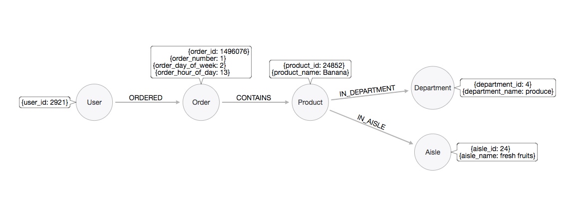
The nodes represent entities in our system: User, Order, Product, Department and Aisle. The edges represent relationships: ORDERED, CONTAINS, IN_DEPARTMENT and IN_AISLE. The attributes in the nodes represent properties (eg: a User has property "user_id"). Mapping to natural language, we can generally think of nodes as nouns, edges as verbs and properties as adjectives.
In this particular graph, each node type contains the same set of properties (eg: all Orders have an order_id, order_number, order_day_of_week and order_hour_of_day), but one of the interesting properties of graph databases is that it is schema-free. This means that a node can have an arbitrary set of properties. For example, we can have two user nodes, u1 and u2, with u1 having properties such as name, address and phone number, and u2 having properties such as name and email. The concept of a schema-free model also applies to the relationships that exist in the graph.
We will be implementing the property graph model above using Neo4j, arguably the most popular graph database today. The actual creation and querying of the database will be done using the Cypher query language, often thought of as SQL for graphs.
Input Dataset 
Similar to my post on association rules mining, we will once again be using data from Instacart. The datasets can be downloaded from the link below, along with the data dictionary:
“The Instacart Online Grocery Shopping Dataset 2017”, Accessed from https://www.instacart.com/datasets/grocery-shopping-2017 on Oct 10, 2017.
Part 1: Data Preparation 
import pandas as pd
import numpy as np
import sys
# Utility functions

# Returns the size of an object in MB
def size(obj):
    return "{0:.2f} MB".format(sys.getsizeof(obj) / (1000 * 1000))

# Displays dataframe dimensions, size and top 5 records
def inspect_df(df_name, df):
    print('{0} --- dimensions: {1};  size: {2}'.format(df_name, df.shape, size(df)))
    display(df.head())

# Exports dataframe to CSV, the format for loading data into Neo4j
def export_to_csv(df, out):
    df.to_csv(out, sep='|', columns=df.columns, index=False)
A. Load user order data 
Data from Instacart contains 3-99 orders per user. Inspecting the distribution of number of orders per user, we see that users place 16 orders on average, with 75% of the user base placing at least 5 orders. For demonstration purposes, we will be running collaborative filtering on a random sample of 100 users who purchased at least 5 orders.
min_orders   = 5     # minimum order count per user
sample_count = 100   # number of users to select randomly

# Load data from evaluation set "prior" (please see data dictionary for definition of 'eval_set')
order_user           = pd.read_csv('orders.csv')
order_user           = order_user[order_user['eval_set'] == 'prior']

# Get distribution of number of orders per user
user_order_count     = order_user.groupby('user_id').agg({'order_id':'count'}).rename(columns={'order_id':'num_orders'}).reset_index()
print('Distribution of number of orders per user:')
display(user_order_count['num_orders'].describe())

# Select users who purchased at least 'min_orders'
user_order_atleast_x = user_order_count[user_order_count['num_orders'] >= min_orders]

# For reproducibility, set seed before taking a random sample
np.random.seed(1111)
user_sample          = np.random.choice(user_order_atleast_x['user_id'], sample_count, replace=False)

# Subset 'order_user' to include records associated with the 100 randomly selected users
order_user           = order_user[order_user['user_id'].isin(user_sample)]
order_user           = order_user[['order_id','user_id','order_number','order_dow','order_hour_of_day']]
inspect_df('order_user', order_user)
B. Load order details data 
# Load orders associated with our 100 selected users, along with the products contained in those orders
order_product = pd.read_csv('order_products__prior.csv')
order_product = order_product[order_product['order_id'].isin(order_user.order_id.unique())][['order_id','product_id']]
inspect_df('order_product', order_product)
C. Load product data 
# Load products purchased by our 100 selected users
products = pd.read_csv('products.csv')
products = products[products['product_id'].isin(order_product.product_id.unique())]
inspect_df('products', products)
D. Load aisle data 
# Load entire aisle data as it contains the names related to the aisle IDs from the 'products' data
aisles = pd.read_csv('aisles.csv')
inspect_df('aisles', aisles)
E. Load department data 
# Load entire department data as it contains the names related to the department IDs from the 'products' data
departments = pd.read_csv('departments.csv')
inspect_df('departments', departments)
F. Export dataframes to CSV, which in turn will be loaded into Neo4j 
export_to_csv(order_user,    '~/neo4j_instacart/import/neo4j_order_user.csv')
export_to_csv(order_product, '~/neo4j_instacart/import/neo4j_order_product.csv')
export_to_csv(products,      '~/neo4j_instacart/import/neo4j_products.csv')
export_to_csv(aisles,        '~/neo4j_instacart/import/neo4j_aisles.csv')
export_to_csv(departments,   '~/neo4j_instacart/import/neo4j_departments.csv')
Part 2: Create Neo4j Graph Database 
A. Set up authentication and connection to Neo4j 
# py2neo allows us to work with Neo4j from within Python
from py2neo import authenticate, Graph

# Set up authentication parameters
authenticate("localhost:7474", "neo4j", "xxxxxxxx")

# Connect to authenticated graph database
g = Graph("http://localhost:7474/db/data/")
B. Start with an empty database, then create constraints to ensure uniqueness of nodes 
# Each time this notebook is run, we start with an empty graph database
g.run("MATCH (n) DETACH DELETE n;")

# We drop and recreate our node constraints
g.run("DROP CONSTRAINT ON (order:Order)             ASSERT order.order_id            IS UNIQUE;")
g.run("DROP CONSTRAINT ON (user:User)               ASSERT user.user_id              IS UNIQUE;")
g.run("DROP CONSTRAINT ON (product:Product)         ASSERT product.product_id        IS UNIQUE;")
g.run("DROP CONSTRAINT ON (aisle:Aisle)             ASSERT aisle.aisle_id            IS UNIQUE;")
g.run("DROP CONSTRAINT ON (department:Department)   ASSERT department.department_id  IS UNIQUE;")

g.run("CREATE CONSTRAINT ON (order:Order)           ASSERT order.order_id            IS UNIQUE;")
g.run("CREATE CONSTRAINT ON (user:User)             ASSERT user.user_id              IS UNIQUE;")
g.run("CREATE CONSTRAINT ON (product:Product)       ASSERT product.product_id        IS UNIQUE;")
g.run("CREATE CONSTRAINT ON (aisle:Aisle)           ASSERT aisle.aisle_id            IS UNIQUE;")
g.run("CREATE CONSTRAINT ON (department:Department) ASSERT department.department_id  IS UNIQUE;")
C. Load product data into Neo4j 
query = """
        // Load and commit every 500 records
        USING PERIODIC COMMIT 500
        LOAD CSV WITH HEADERS FROM 'file:///neo4j_products.csv' AS line FIELDTERMINATOR '|'
        WITH line

        // Create Product, Aisle and Department nodes
        CREATE (product:Product {product_id: toInteger(line.product_id), product_name: line.product_name})
        MERGE  (aisle:Aisle {aisle_id: toInteger(line.aisle_id)})
        MERGE  (department:Department {department_id: toInteger(line.department_id)})

        // Create relationships between products and aisles & products and departments
        CREATE (product)-[:IN_AISLE]->(aisle)
        CREATE (product)-[:IN_DEPARTMENT]->(department);
        """

g.run(query)
D. Load aisle data into Neo4j 
query = """
        // Aisle data is very small, so there is no need to do periodic commits
        LOAD CSV WITH HEADERS FROM 'file:///neo4j_aisles.csv' AS line FIELDTERMINATOR '|'
        WITH line

        // For each Aisle node, set property 'aisle_name'
        MATCH (aisle:Aisle {aisle_id: toInteger(line.aisle_id)})
        SET aisle.aisle_name = line.aisle;
        """

g.run(query)
E. Load department data into Neo4j 
query = """
        // Department data is very small, so there is no need to do periodic commits
        LOAD CSV WITH HEADERS FROM 'file:///neo4j_departments.csv' AS line FIELDTERMINATOR '|'
        WITH line

        // For each Department node, set property 'department_name'
        MATCH (department:Department {department_id: toInteger(line.department_id)})
        SET department.department_name = line.department;
        """

g.run(query)
F. Load order details data into Neo4j 
query = """
        // Load and commit every 500 records
        USING PERIODIC COMMIT 500
        LOAD CSV WITH HEADERS FROM 'file:///neo4j_order_product.csv' AS line FIELDTERMINATOR '|'
        WITH line

        // Create Order nodes and then create relationships between orders and products
        MERGE (order:Order {order_id: toInteger(line.order_id)})
        MERGE (product:Product {product_id: toInteger(line.product_id)})
        CREATE (order)-[:CONTAINS]->(product);
        """

g.run(query)
G. Load user order data into Neo4j 
query = """
        // Load and commit every 500 records
        USING PERIODIC COMMIT 500
        LOAD CSV WITH HEADERS FROM 'file:///neo4j_order_user.csv' AS line FIELDTERMINATOR '|'
        WITH line

        // Create User nodes and then create relationships between users and orders
        MERGE (order:Order {order_id: toInteger(line.order_id)})
        MERGE (user:User   {user_id:  toInteger(line.user_id)})

        // Create relationships between users and orders, then set Order properties
        CREATE(user)-[o:ORDERED]->(order)
        SET order.order_number = toInteger(line.order_number),
            order.order_day_of_week = toInteger(line.order_dow),
            order.order_hour_of_day = toInteger(line.order_hour_of_day);
        """

g.run(query)
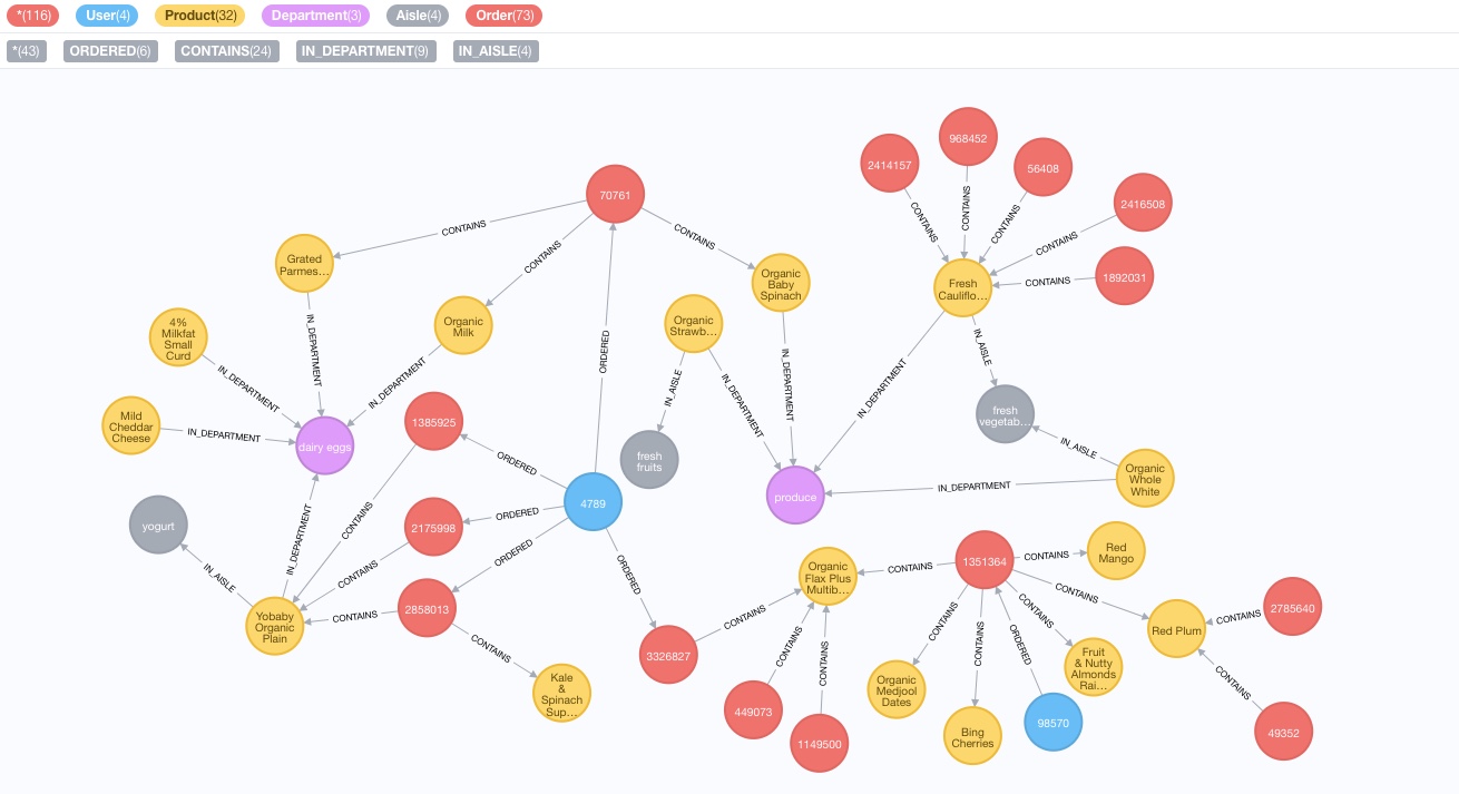
H. What our graph looks like 
This is what the nodes and relationships we have created look like in Neo4j for a small subset of the data. Please use the legend on the top left corner only to determine the colours associated with the different nodes (ie: ignore the numbers).
Part 3: Implement User-User Collaborative Filtering Algorithm 
# Implements user-user collaborative filtering using the following steps:
#   1. For each user pair, compute Jaccard index
#   2. For each target user, select top k neighbours based on Jaccard index
#   3. Identify products purchased by the top k neighbours that have not been purchased by the target user
#   4. Rank these products by the number of purchasing neighbours
#   5. Return the top n recommendations for each user

def collaborative_filtering(graph, neighbourhood_size, num_recos):

    query = """
           // Get user pairs and count of distinct products that they have both purchased
           MATCH (u1:User)-[:ORDERED]->(:Order)-[:CONTAINS]->(p:Product)<-[:CONTAINS]-(:Order)<-[:ORDERED]-(u2:User)
           WHERE u1 <> u2
           WITH u1, u2, COUNT(DISTINCT p) as intersection_count

           // Get count of all the distinct products that they have purchased between them
           MATCH (u:User)-[:ORDERED]->(:Order)-[:CONTAINS]->(p:Product)
           WHERE u in [u1, u2]
           WITH u1, u2, intersection_count, COUNT(DISTINCT p) as union_count

           // Compute Jaccard index
           WITH u1, u2, intersection_count, union_count, (intersection_count*1.0/union_count) as jaccard_index

           // Get top k neighbours based on Jaccard index
           ORDER BY jaccard_index DESC, u2.user_id
           WITH u1, COLLECT(u2)[0..{k}] as neighbours
           WHERE LENGTH(neighbours) = {k}                                              // only want users with enough neighbours
           UNWIND neighbours as neighbour
           WITH u1, neighbour

           // Get top n recommendations from the selected neighbours
           MATCH (neighbour)-[:ORDERED]->(:Order)-[:CONTAINS]->(p:Product)             // get all products bought by neighbour
           WHERE not (u1)-[:ORDERED]->(:Order)-[:CONTAINS]->(p)                        // which target user has not already bought
           WITH u1, p, COUNT(DISTINCT neighbour) as cnt                                // count neighbours who purchased product
           ORDER BY u1.user_id, cnt DESC                                               // sort by count desc
           RETURN u1.user_id as user, COLLECT(p.product_name)[0..{n}] as recos         // return top n products
           """

    recos = {}
    for row in graph.run(query, k=neighbourhood_size, n=num_recos):
        recos[row[0]] = row[1]

    return recos
Part 4: Execute User-User Collaborative Filtering 
Our collaborative filtering function expects 3 parameters: a graph database, the neighbourhood size and the number of products to recommend to each user. A reminder that our graph database, g, contains nodes and relationships pertaining to user orders. And as previously discussed, we have chosen k=10 as the neighbourhood size and n=10 as the number of products to recommend to each of our users. We now invoke our collaborative filtering function using these parameters.
%%time
recommendations = collaborative_filtering(g,10,10)
display(recommendations)
As can be seen above, our collaborative filtering function returns a dictionary of users and their top 10 recommended products. To see how we arrived at the output above, let's break down our function using a speficic example, user 4789. For reference, below are the products that this user has been recommended:
recommendations[4789]
The first main component of our collaborative filtering function identifies the top 10 neighbours for user 4789. It does so by creating user pairs, where u1 is always user 4789 and u2 is any other user who has purchased products that u1 has purchased. It then computes the Jaccard index for each user pair, by taking the number of distinct products that u1 and u2 have purchased in common (intersection_count) and dividing it by the number of distinct products that are unique to each user (union_count). The 10 users with the highest Jaccard index are selected as user 4789's neighbourhood.
query = """
        // Get count of all distinct products that user 4789 has purchased and find other users who have purchased them
        MATCH (u1:User)-[:ORDERED]->(:Order)-[:CONTAINS]->(p:Product)<-[:CONTAINS]-(:Order)<-[:ORDERED]-(u2:User)
        WHERE u1 <> u2
          AND u1.user_id = {uid}
        WITH u1, u2, COUNT(DISTINCT p) as intersection_count

        // Get count of all the distinct products that are unique to each user
        MATCH (u:User)-[:ORDERED]->(:Order)-[:CONTAINS]->(p:Product)
        WHERE u in [u1, u2]
        WITH u1, u2, intersection_count, COUNT(DISTINCT p) as union_count

        // Compute Jaccard index
        WITH u1, u2, intersection_count, union_count, (intersection_count*1.0/union_count) as jaccard_index

        // Get top k neighbours based on Jaccard index
        ORDER BY jaccard_index DESC, u2.user_id
        WITH u1, COLLECT([u2.user_id, jaccard_index, intersection_count, union_count])[0..{k}] as neighbours

        WHERE LENGTH(neighbours) = {k}                // only want to return users with enough neighbours
        RETURN u1.user_id as user, neighbours
        """

neighbours = {}
for row in g.run(query, uid=4789, k=10):
    neighbours[row[0]] = row[1]

print("Labels for user 4789's neighbour list: user_id, jaccard_index, intersection_count, union count")
display(neighbours)
The second main component of our collaborative filtering function generates recommendations for user 4789 using the neighbours identified above. It does so by considering products that the neighbours have purchased which user 4789 has not already purchased. The function then counts the number of neighbours who have purchased each of the candidate products. The 10 products with the highest neighbour count are selected as recommendations for user 4789.
%%time
query = """
        // Get top n recommendations for user 4789 from the selected neighbours
        MATCH (u1:User),
              (neighbour:User)-[:ORDERED]->(:Order)-[:CONTAINS]->(p:Product)        // get all products bought by neighbour
        WHERE u1.user_id = {uid}
          AND neighbour.user_id in {neighbours}
          AND not (u1)-[:ORDERED]->(:Order)-[:CONTAINS]->(p)                        // which u1 has not already bought

        WITH u1, p, COUNT(DISTINCT neighbour) as cnt                                // count times purchased by neighbours
        ORDER BY u1.user_id, cnt DESC                                               // and sort by count desc
        RETURN u1.user_id as user, COLLECT([p.product_name,cnt])[0..{n}] as recos
        """

recos = {}
for row in g.run(query, uid=4789, neighbours=[42145,138203,87350,49441,187754,180461,120660,107931,73477,154852], n=10):
    recos[row[0]] = row[1]

print("Labels for user 4789's recommendations list: product, number of purchasing neighbours")
display(recos)
Part 5: Evaluating Recommender Performance 
If we were to actually integrate our recommender system in to a production environment, we would need a way to measure its performance. As mentioned, in the context of a user check-out application for an online grocer, the goal is to increase basket size, by surfacing a short list of products that are as relevant as posssible to the user. For this particular application, we could choose precision as our metric for evaluating our recommender's performance. Precision is computed as the proportion of products that the user actually purchased, out of all the products that user has been recommended. To determine overall recommender performance, average precision can be calculated using the precision values for all the users in the system.
Conclusion 
We have demonstrated how to build a user-based recommender system leveraging the principles of user-user collaborative filtering. We've discussed the key concepts underlying this algorithm, from identifying neighbourhoods using a similarity metric, to generating recommendations for a user based on its neighbours' preferences. In addition, we have shown how easy and intuitive modeling connected data can be with a graph database. One final point worth noting: in real world applications, we may want to implement non-personalized recommendation strategies for users who are new to the system and those who have not yet made sufficient purchases. Strategies may include recommending top selling products for new users, and for the latter group, products identified to have high affinity with other products that the user has already purchased. This can be done through association rules mining, also known as market basket analysis.